Speeding up an OLS regression in R

Yesterday a colleague told me that he was surprised by the speed differences of R, Julia and Stata when estimating a simple linear model for a large number of observations (10 million). Julia and Stata had very similar results, although Stata was faster. But both Julia and Stata were substantially faster than R. He is an expert and long time Stata user and was sceptical about the performance difference. I was also surprised. My experience is that R is usually fast, for interpreted language, and most procedures that are computationally intensive are developed in a compiled language like C, Fortran or C++, reducing any performance penalty.

The model he was trying to estimate was the following:

RNGkind(kind = "Mersenne-Twister")
set.seed(42)
nobs <- 10000000
test_data <- data.frame(y = runif(nobs),
                        x1 = runif(nobs),
                        x2 = runif(nobs))

system.time(
  fit <- lm(y ~ 1 + x1 + x2, data = test_data)
)

##    user  system elapsed 
##  14.612   0.820  15.479

The result is not unsatisfactory in itself, quite the contrary, and only in some particular settings (like bootstrapping) this would be a problem, but the relative performance to Stata was not that great. On his machine, this was about three times slower than Stata. I know that lm() function does have a lot of overhead, so I tried other approaches.

Let’s start by loading a few packages:

library(speedglm)

## Loading required package: Matrix

## Loading required package: MASS

library(RcppEigen)
library(ggplot2)
library(microbenchmark)

I’m using the speedlm() and speedlm.fit() functions from the speedglm package, and the fastLm() function from the RcppEigen package. I need the ggplot2 and microbenchmark packages to make a performance comparison and plotting the results.

Since some functions take the input data as a matrix instead of a data frame, I’m also creating matrix representation of the data:

x <- as.matrix(cbind(1, test_data[, 2:3]))
y <- test_data$y

Now the comparison:

bench <- microbenchmark(
  fit_lm <-  lm(y ~ 1 + x1 +  x2, data = test_data),
  fit_lsfit <- lsfit(x, y, intercept = FALSE),
  fit_lm.fit <- lm.fit(x, y),
  fit_.lm.fit <- .lm.fit(x, y),
  fit_speedlm_df <- speedlm(y ~ 1 + x1 + x2, data = test_data),
  fit_speedlm_matrix <- speedlm.fit(y = y, X = x, intercept = FALSE),
  fit_fastLM_df <- fastLm(y ~ 1 + x1 + x2, data = test_data),
  fit_fastLM_matrix <- fastLm(x, y),
  times = 10
)

I’m comparing the lm() function against the lsfit(), lm.fit(), .lm.fit() functions from base R, the speedlm() and speedlm.fit() from the speedglm package, and finally the fastLm() function from the RcppEigen packages.¹

Before discussing the results, a word of caution. This is a simple toy example. The effective performance of these functions will depend on the problem itself, the operating system, the math libraries that R is using, the CPU of the machine, and the sustained maximum CPU clock of the computer, among other things. Moreover the lm.fit() and .lm.fit() functions shouldn’t be used directly, as stated by the R documentation.²

First, let’s check if the results are the same for all approaches:

all.equal(fit_lm$coefficients, 
          fit_lsfit$coefficients,
          fit_lm.fit$coefficients,
          fit_.lm.fit$coefficients,
          fit_speedlm_df$coefficients,
          fit_speedlm_matrix$coefficients,
          fit_fastLM_df$coefficients,
          fit_fastLM_matrix$coefficients,
          check.names = FALSE)

## [1] TRUE

Then we can compare the efficiency of the different methods:

autoplot(bench, log=TRUE)

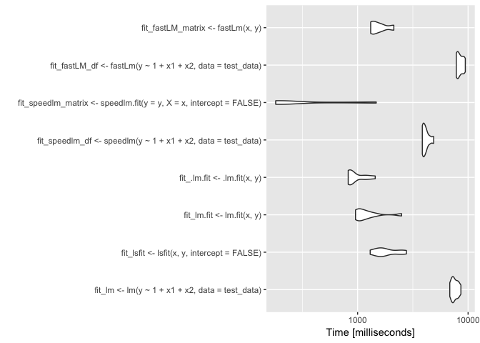
bench

## Unit: milliseconds
##                                                                expr
##                     fit_lm <- lm(y ~ 1 + x1 + x2, data = test_data)
##                         fit_lsfit <- lsfit(x, y, intercept = FALSE)
##                                          fit_lm.fit <- lm.fit(x, y)
##                                        fit_.lm.fit <- .lm.fit(x, y)
##        fit_speedlm_df <- speedlm(y ~ 1 + x1 + x2, data = test_data)
##  fit_speedlm_matrix <- speedlm.fit(y = y, X = x, intercept = FALSE)
##          fit_fastLM_df <- fastLm(y ~ 1 + x1 + x2, data = test_data)
##                                   fit_fastLM_matrix <- fastLm(x, y)
##        min        lq      mean    median        uq      max neval
##  6828.9345 7146.6856 7591.7983 7390.2312 8099.4330 8609.801    10
##  1299.4915 1560.6033 1872.1942 1702.5058 2370.6262 2766.618    10
##   957.6946  995.4642 1260.5417 1097.8551 1278.9813 2502.580    10
##   821.9108  846.9022  976.0173  863.4897 1112.1696 1443.480    10
##  3852.0476 3905.1333 4145.0058 4061.1713 4250.1291 4880.512    10
##   181.3953  182.2440  492.0430  207.2382  603.4584 1474.690    10
##  7826.8584 7937.1581 8464.2897 8307.2791 9106.6024 9436.472    10
##  1313.2983 1361.3758 1588.5146 1476.4634 1685.5722 2127.451    10

The x-axis of the plot is in logarithm scale. The results show that the computational speed can be substantially different and faster than the lm() function. One method, in particular, the fastLm() function using matrices as an input, resulted in a very small computational time (about 0.2 seconds). By the way, this result is much faster than Stata.

This simple example illustrates that performance comparisons between different statistical software are hard to do. They will be dependent on our level of expertise in each language. I’m my opinion performance is just one dimension we should take into account when choosing a software/language. The depth and breath of R, and it’s data manipulation tools more than compensate for any performance penalty from using an interpreted language. In any case, when I hit a performance bottleneck it is easy in R to integrate C++ or to parallelise the code.